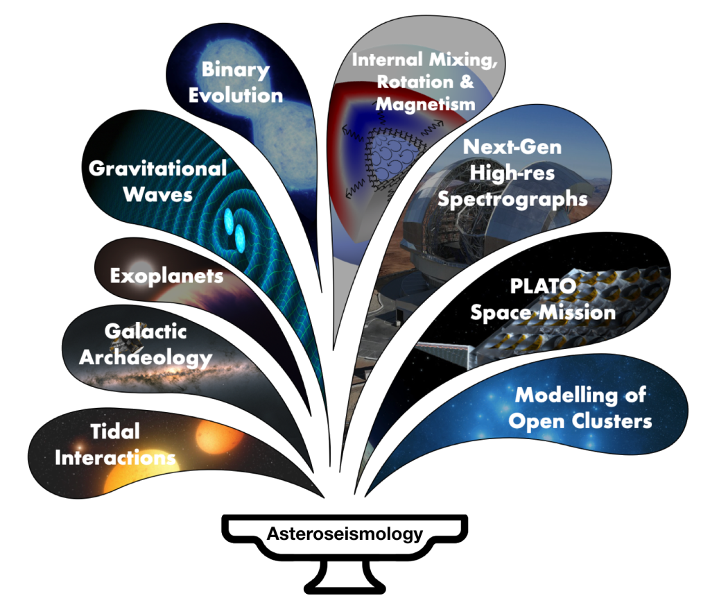

3 Main Uses:
- Fundamental Properties
- Dynamic and Activity
- Internal Structure
Center for Astrophysics | Harvard &
Smithsonian;
January 28, 2025
physics of stellar interiors
quantitative
astronomy & astrophysics
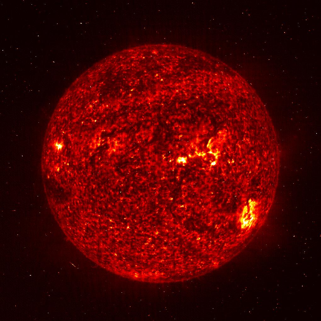
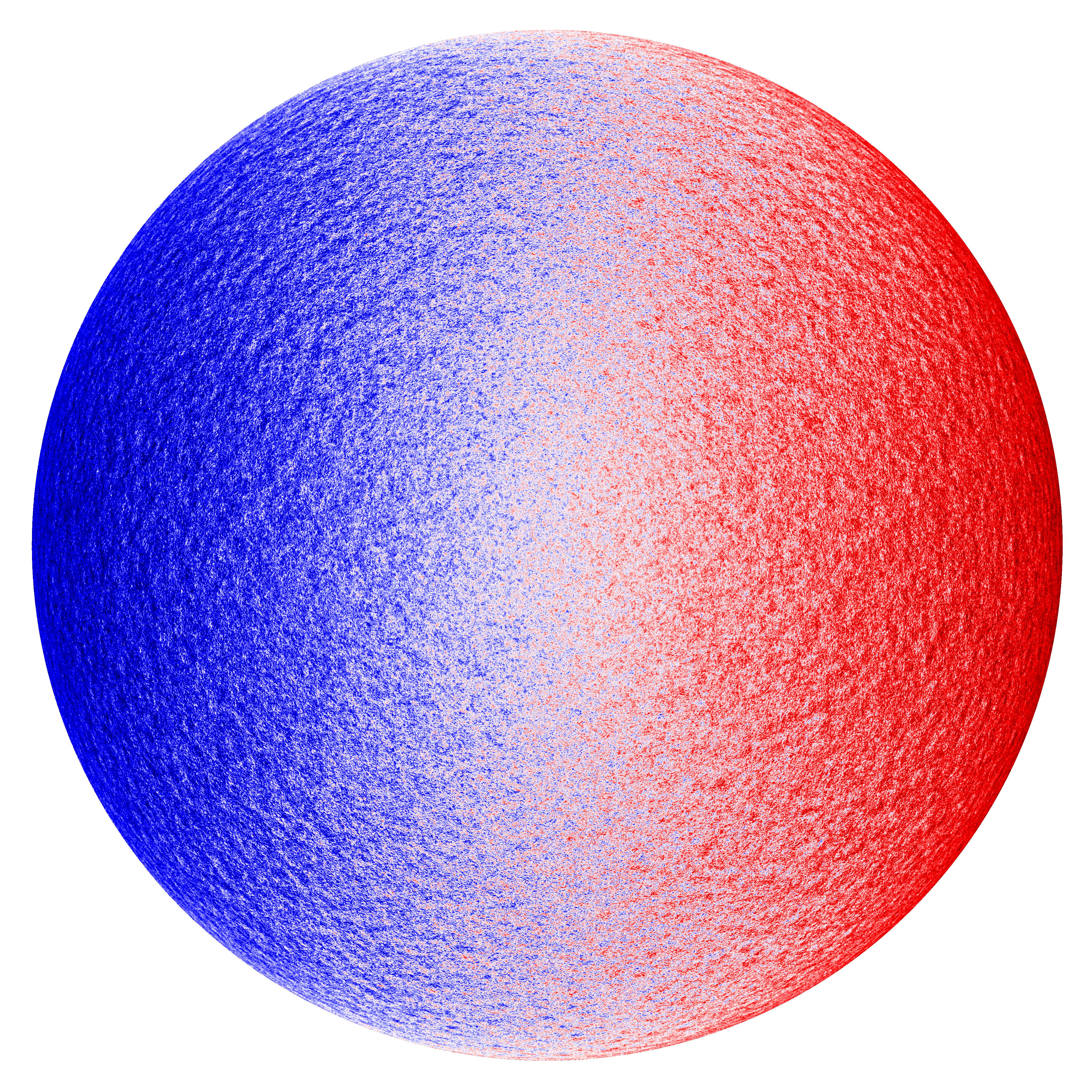
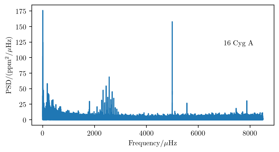
\(\ell = 0\) MDI Doppler velocities


Power spectra of MDI dopplergrams
\[ \begin{aligned} {\Delta\nu_\odot} &\sim 135\ \mathrm{\mu Hz} \\ {\nu_{\text{max},\odot}} &\sim 3090\ \mathrm{\mu Hz} \end{aligned} \]
(roughly 5-minute oscillations)
p-mode frequencies satisfy \(\nu_{n\ell} \sim \Delta\nu\left(n + {\ell \over 2} + \epsilon_\ell(\nu)\right) + \mathcal{O}(1/\nu)\)
Stochastic,
broad-band
excitation
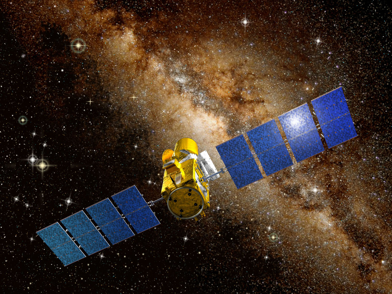
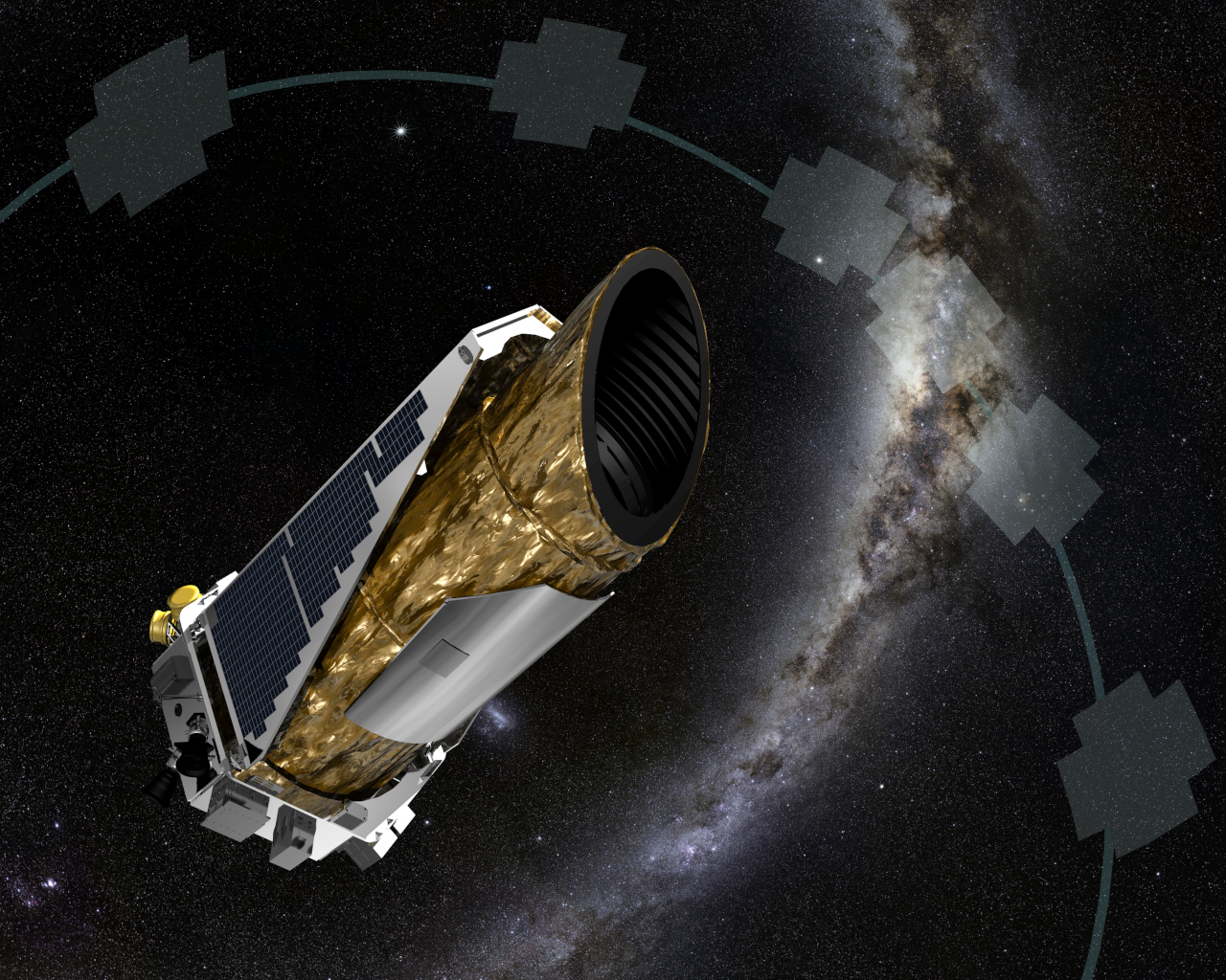
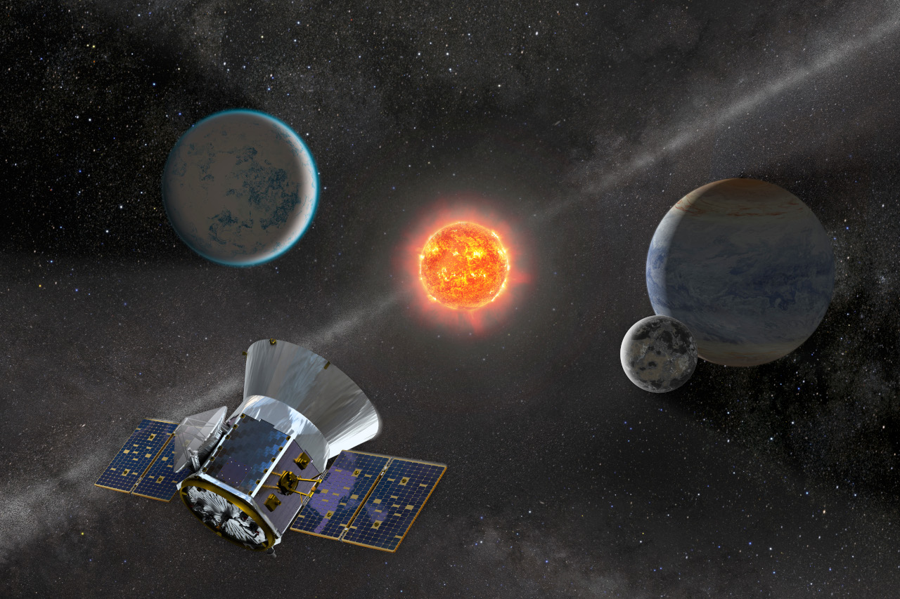
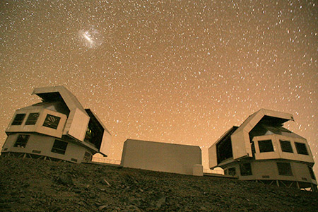
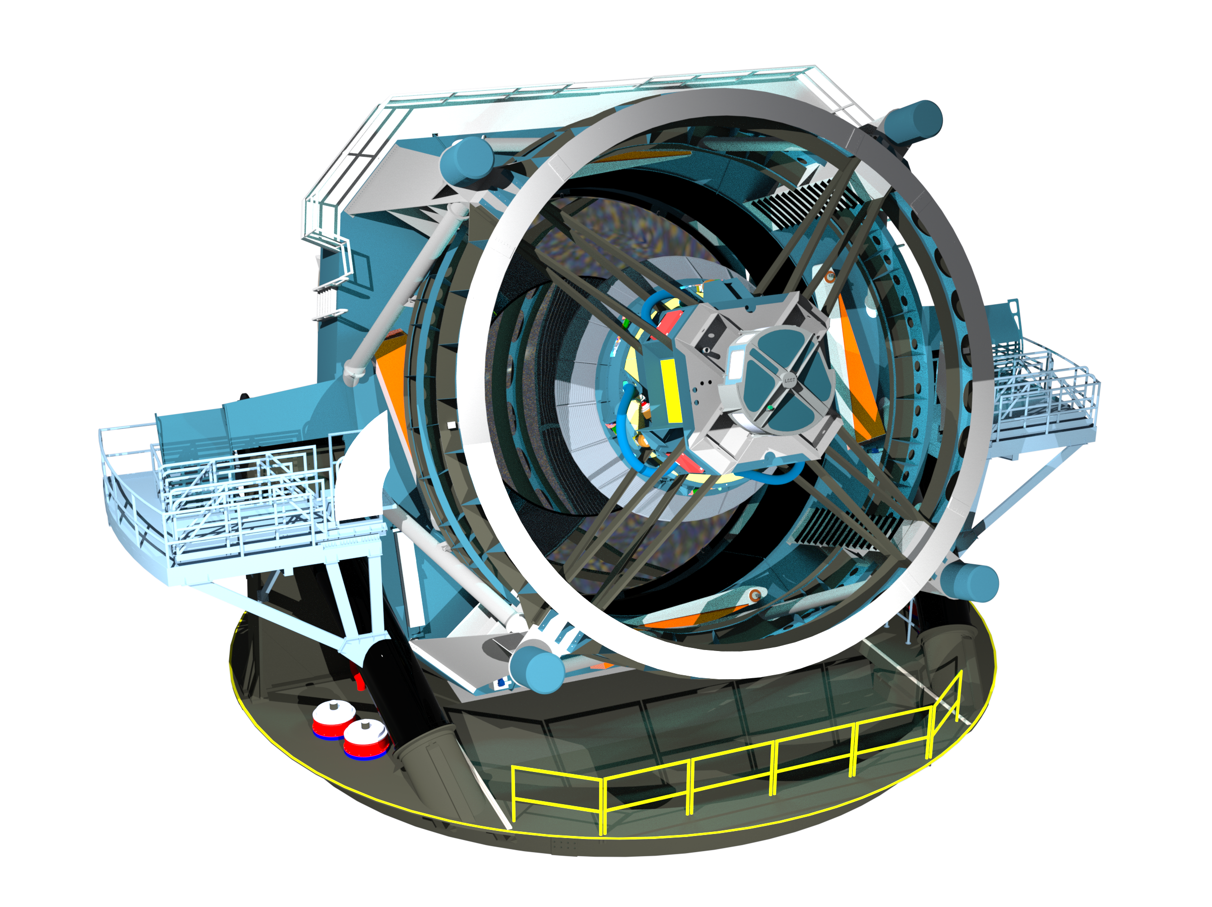
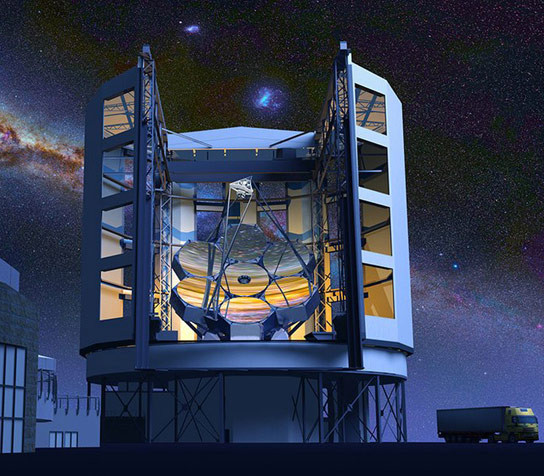
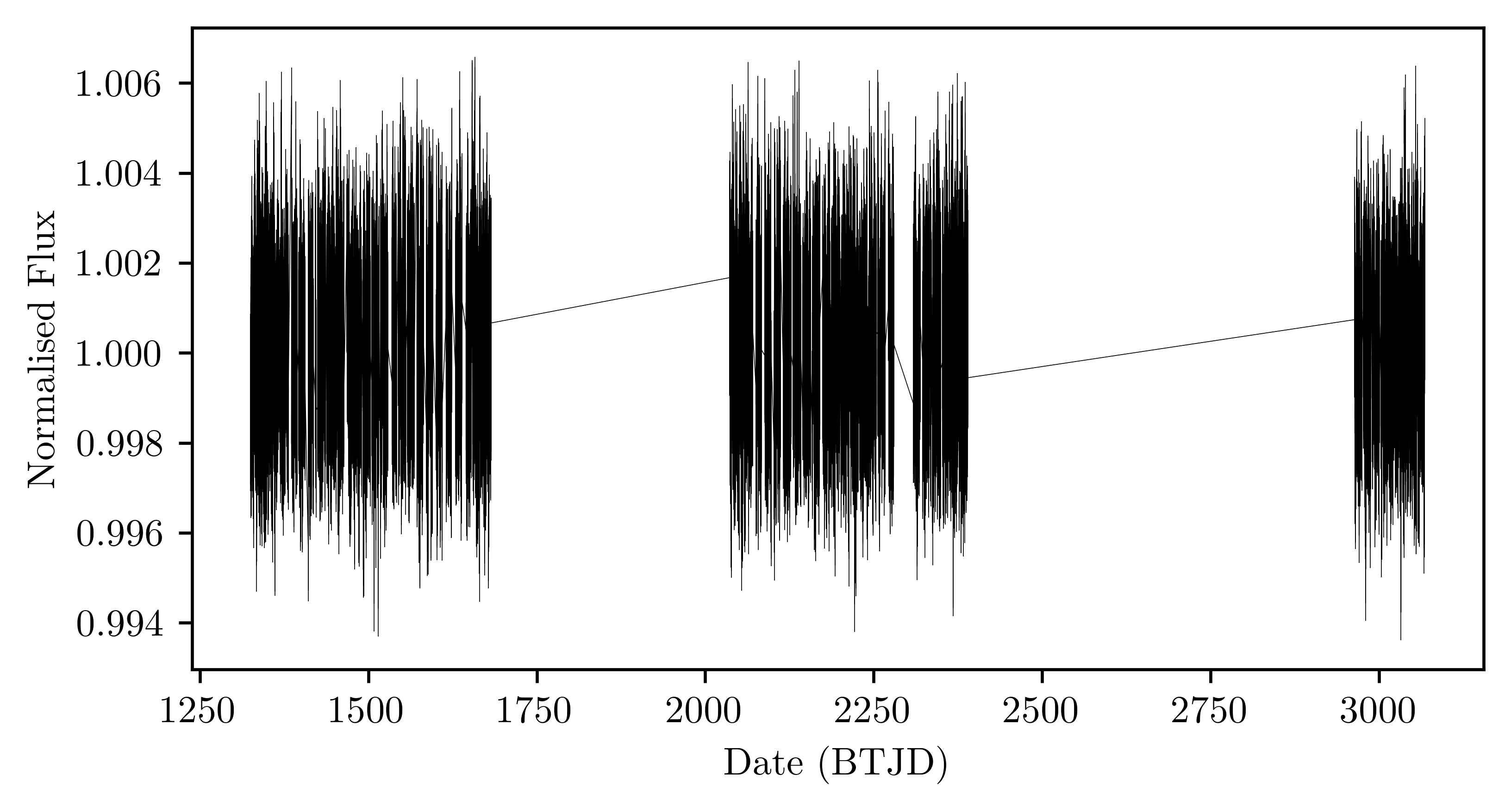
Telescopes can only point at one star at time…
Required photometric stability not achievable from ground


Hare “Zebedee”, Cunha+ incl. Ong (2021);
HPC & pipeline: Ong+ 2021a


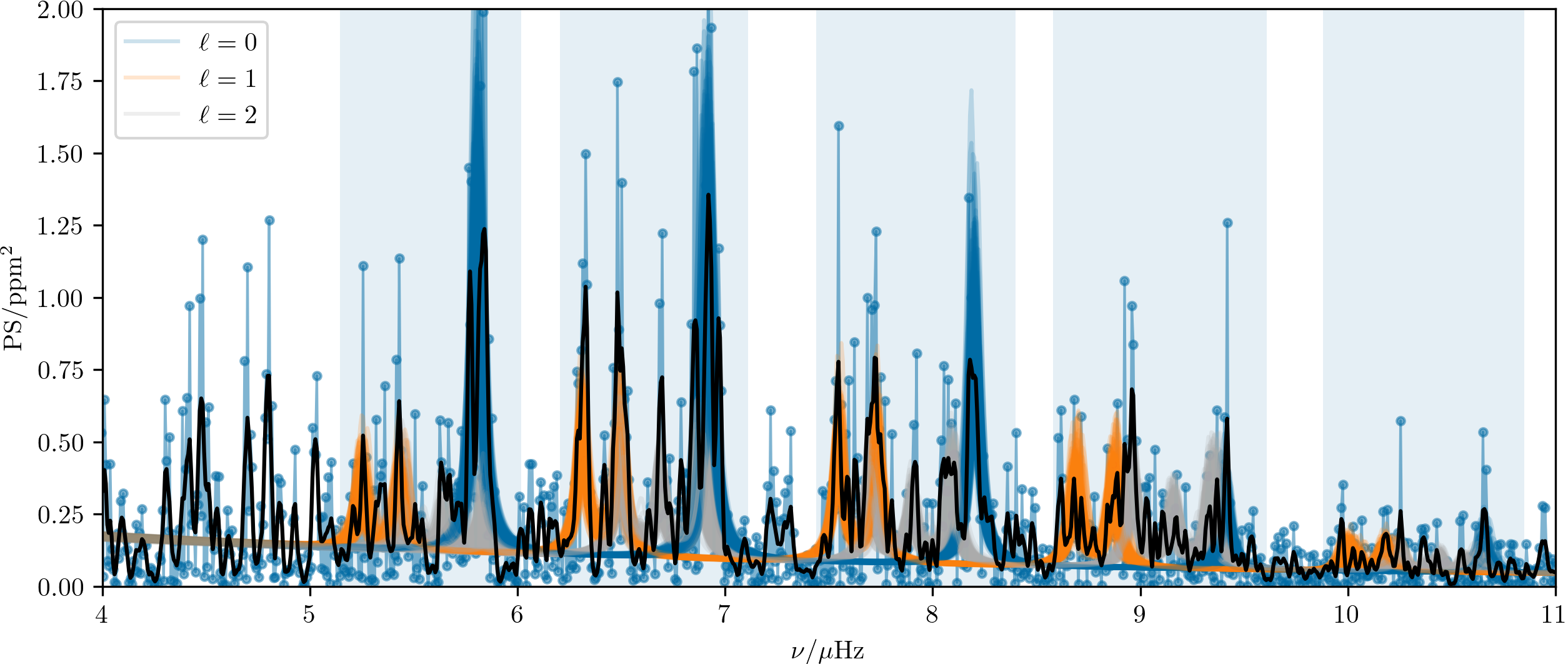
Precise measurements of field stars: \[ {\sigma_R \over R} \lesssim 2 \%;\ {\sigma_M \over M} \lesssim 5 \%;\ \sigma_\text{Age} \lesssim 0.4\ \mathrm{Gyr} \]
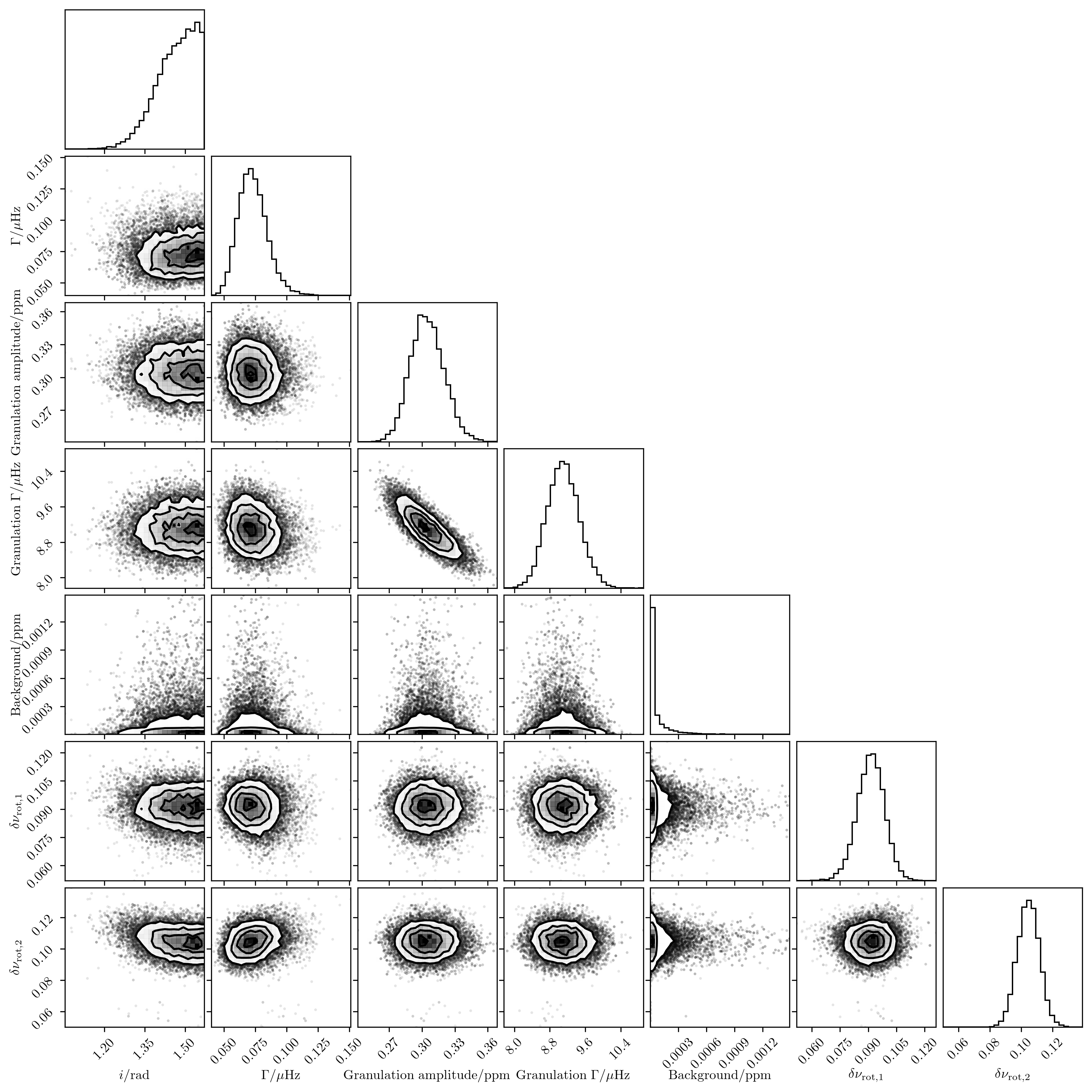
Rotational inversions constrain differential rotation
(e.g. Backus & Gilbert 1968; Gough 1985;
Pijpers & Thompson 1992; Schunker 2016;
Ong 2024 etc.)

(e.g. Ong et al. 2024, Ong 2025)
Probes of the internal states of stars … now return constraints on stellar structure previously only theorized. —Astro 2020
Decadal Survey
(e.g. Bellinger+ 2017,2019;Ong & Basu
2019a,b;
Lindsay, Ong, Basu 2022†, 2023†,
2024†;
Vanlaer+ 2023; Buchele+ 2024, 2025)

†: mentoree paper
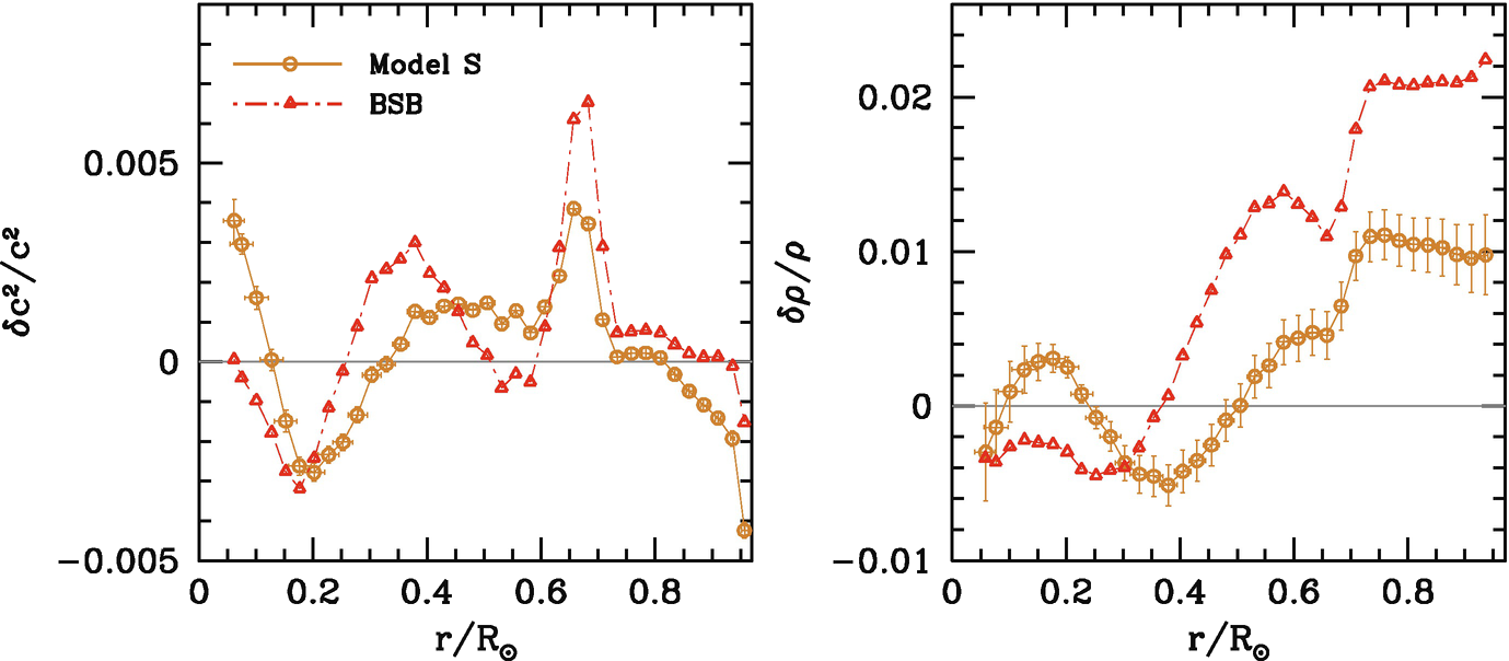
Bellinger+ 2019
Relative difference in isothermal sound speed
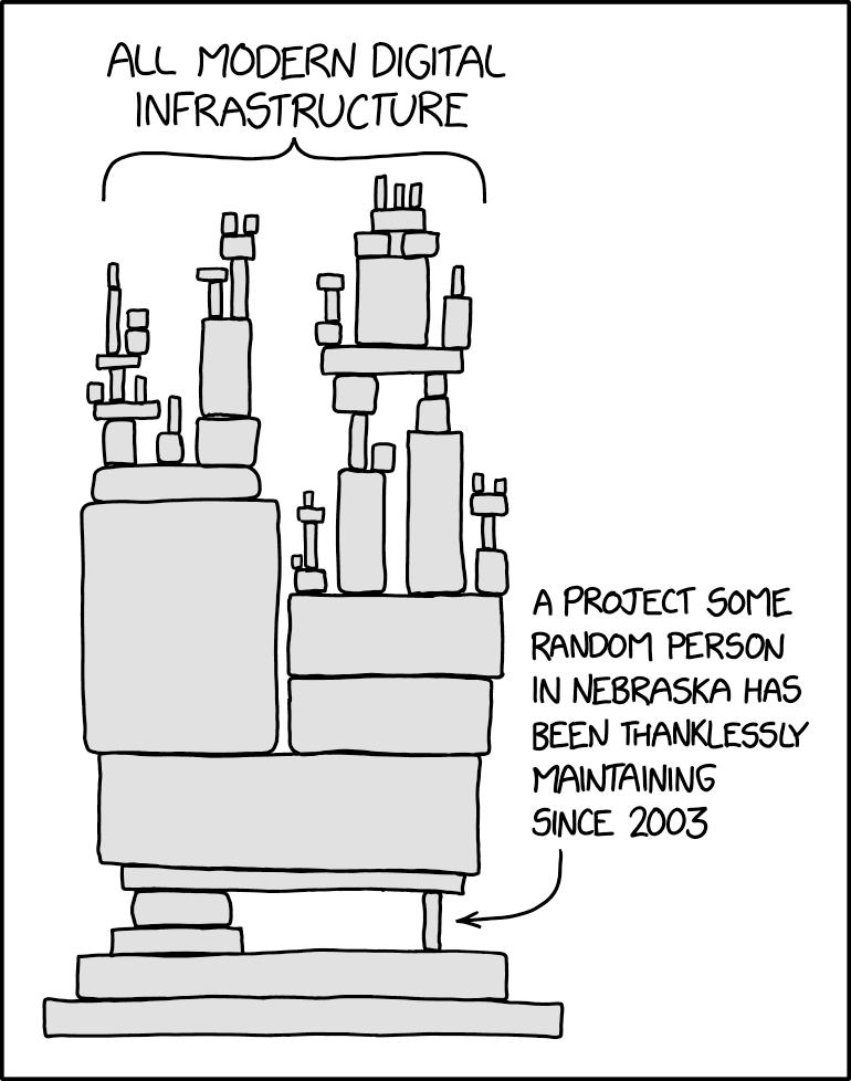
We are drowning in data.
big data deluge
physical interpretation
analytic theory
computational technique
statistical methodology
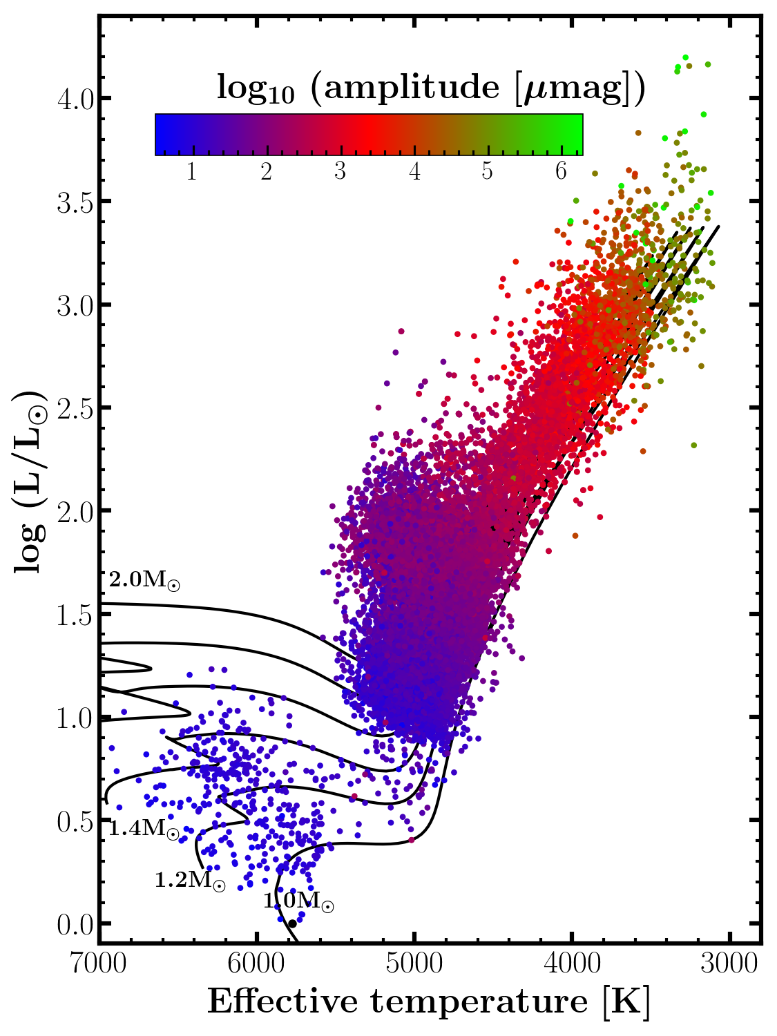
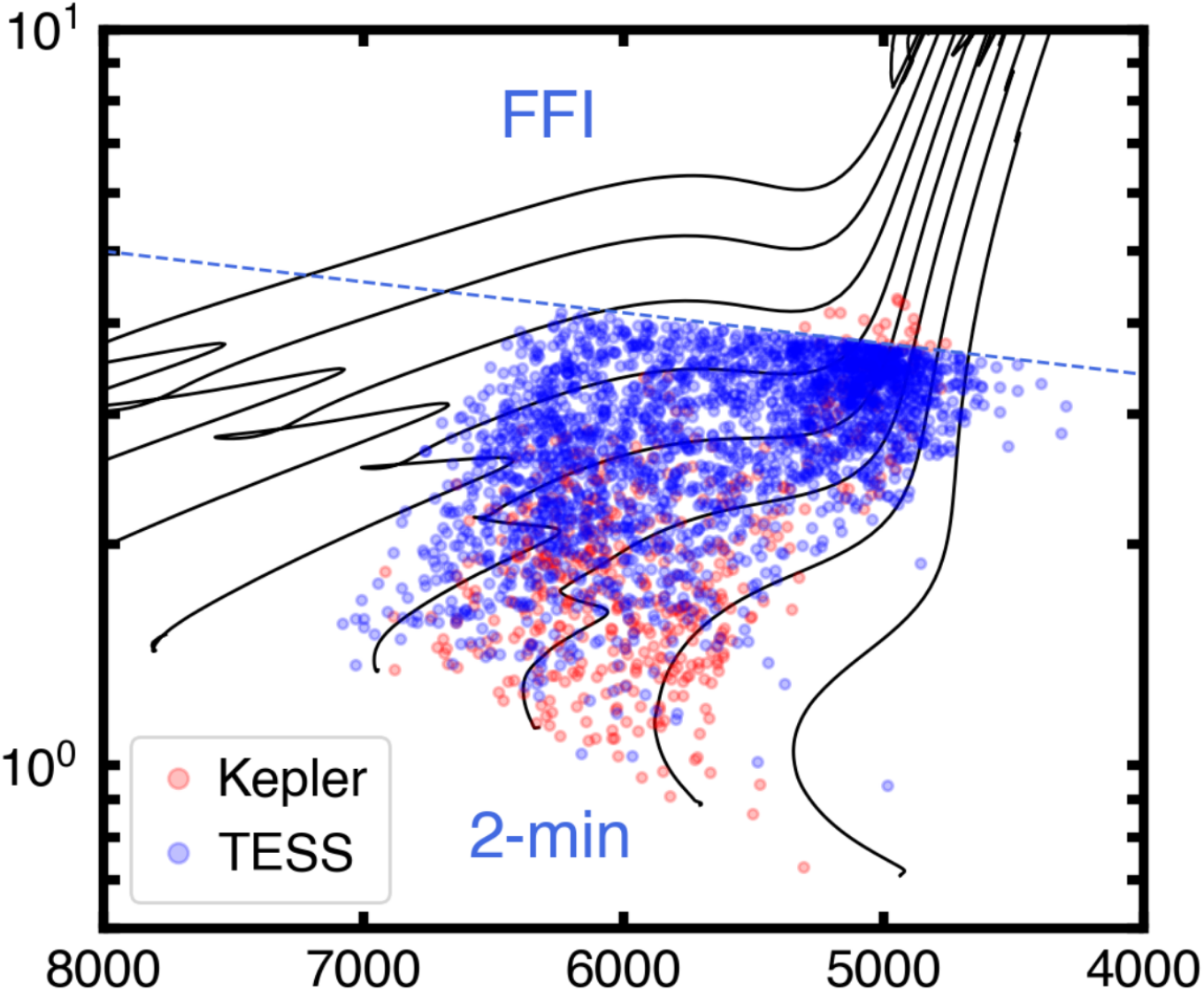
Evolved stars dominate our asteroseismic sample.
(e.g. only \(\sim 100\) Kepler main-sequence stars)
\[\large V_\text{osc} \sim L/M\]
\(T_\text{eff}/\mathrm{K}\)
\(R/R_\odot\)

g-mode Period Spacing \(\Delta\Pi_1/\mathrm{s}\)
p-mode Frequency Spacing \(\Delta\nu/\mu\mathrm{Hz}\)
from Mosser+ (2014)
Single-star electron degeneracy sequence:
deviations → merger remnants?
(Rui and Fuller 2021, Deheuvels+ 2021)
clump stars
first-ascent RGs


(proxy for age \(\to\))
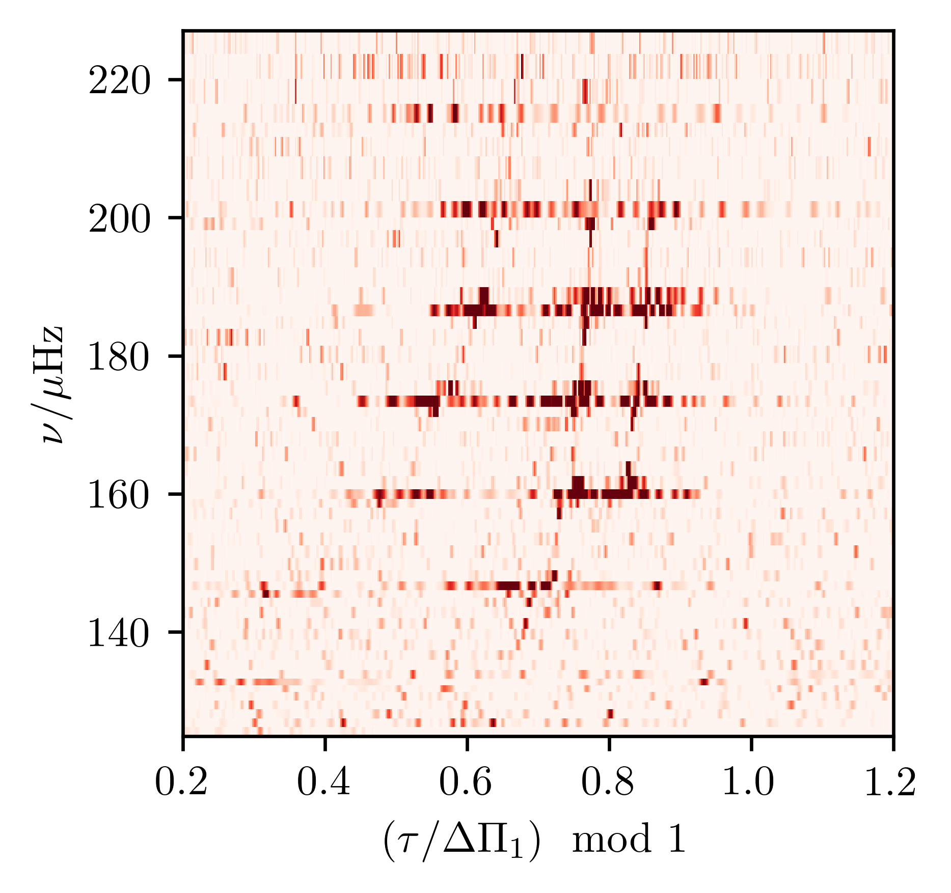
Mixed modes exhibit
avoided crossings
between underlying p- and
g-modes.


\[{c_s^2 k_r^2 \sim \omega^2 \left(1 - {{\color{blue} S_\ell}^2 \over \omega^2}\right)\left(1 - {{\color{darkorange}N}^2 \over \omega^2}\right)}\]
\[\small N^2 = {- g}\left.{\partial \log \rho \over \partial s}\right|_P{\mathrm d s \over \mathrm d r}\] entropy gradient (\(=0\) in CZ)
\[\small S_\ell^2 = c_s^2 k_h^2 = {\ell(\ell+1) c_s^2 \over r^2}\] wave angular momentum
\[\Large \omega_-^2 \sim N^2 {k_h^2 \over |\mathbf{k}|^2}\]
\[{\color{red} \omega_g < N, S_\ell}\]
\[\Large \omega_+^2 \sim c_s^2 |\mathbf{k}|^2\]
\[{\color{gray} \omega_p > S_\ell, N}\]
Brute-force numerical solution (quantitative)
vs
JWKB approximation (qualitative)

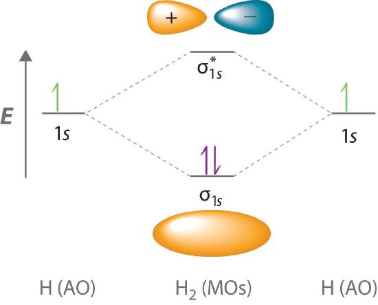
\[\Large \hat H \left|n\right> = \left(\hat T + \hat V\right)\left|n\right> = E_n \left|n\right>\]


\[\large {\color{blue}{\hat H_1}} \left|n\right> = \left(\hat T + \hat V_1\right)\left|n\right> = {\color{blue}E_n \left|n\right>}\]
\[\large {\color{orange}{\hat H_2}} \left|n\right> = \left(\hat T + \hat V_2\right)\left|n\right> = {\color{orange}E_n \left|n\right>}\]
\[\huge \hat H = \hat T + \hat V_1 + \hat V_2 = {\color{blue}{\hat H_1}} + \hat V_2 = \hat V_1 + {\color{orange}{\hat H_2}}\]


\[\Large \hat{\mathcal{L}} \xi_n = -\omega_n^2 \xi_n\]
\[\Large \hat{\mathcal{L}} = {\color{red}\hat{\mathcal{L}}_\gamma} + \hat{\mathcal{R}}_\gamma\]
\[\Large {\color{red}\hat{\mathcal{L}}_\gamma \xi_{\gamma,n} = -\omega^2_{\gamma,n}\xi_{\gamma,n}}\]
\[\Large \hat{\mathcal{L}} = \hat{\mathcal{R}}_\pi + {\color{grey}\hat{\mathcal{L}}_\pi}\]
\[\Large {\color{grey}\hat{\mathcal{L}}_\pi \xi_{\pi,n} = -\omega^2_{\pi,n}\xi_{\pi,n}}\]
\[\Large \hat{\mathcal{L}} = {\color{grey}\hat{\mathcal{L}}_\pi} + \hat{\mathcal{R}}_\pi = \hat{\mathcal{R}}_\gamma + {\color{red}\hat{\mathcal{L}}_\gamma}\]
\[\Large \xi_\text{mixed} \sim {\color{grey}c_\pi \xi_\pi} + {\color{red}c_\gamma \xi_\gamma}\]
Li et al. Nat. 2022:
Asymmetric splittings probe
core magnetic fields
(Li+ 2023, Deheuvels+ 2023;
Rui, Ong, Mathis, 2024†)
Population studies
of rotation vs. magnetism
(Hatt, Ong, et al., 2024†)


\[\scriptsize \delta \nu_{\text{mag}, g, \ell=1} \sim {m^2 \over \nu^3}\]

†: mentoree paper


 Saunders et
al. 2024
Saunders et
al. 2024


Ong 2025

From Huber et al. 2013
Ong 2025


Probing the star-planet connection, and non-canonical evolution
e.g. Ong 2025;
Ong et al. 2024;
Hon et al. (incl Ong) Nat. 2023
(also incl. Ong: Huber+ 2019, 2022; …)
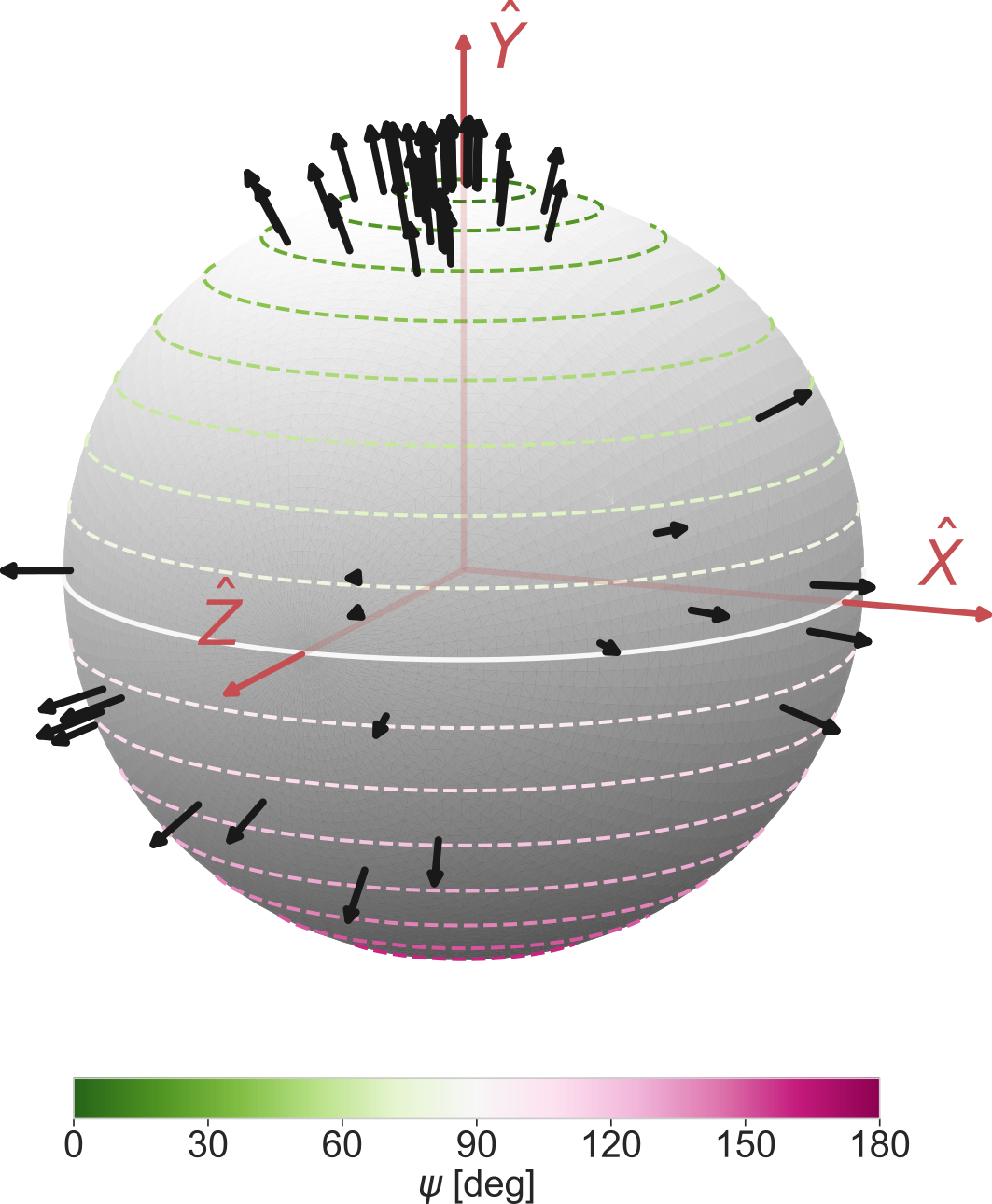
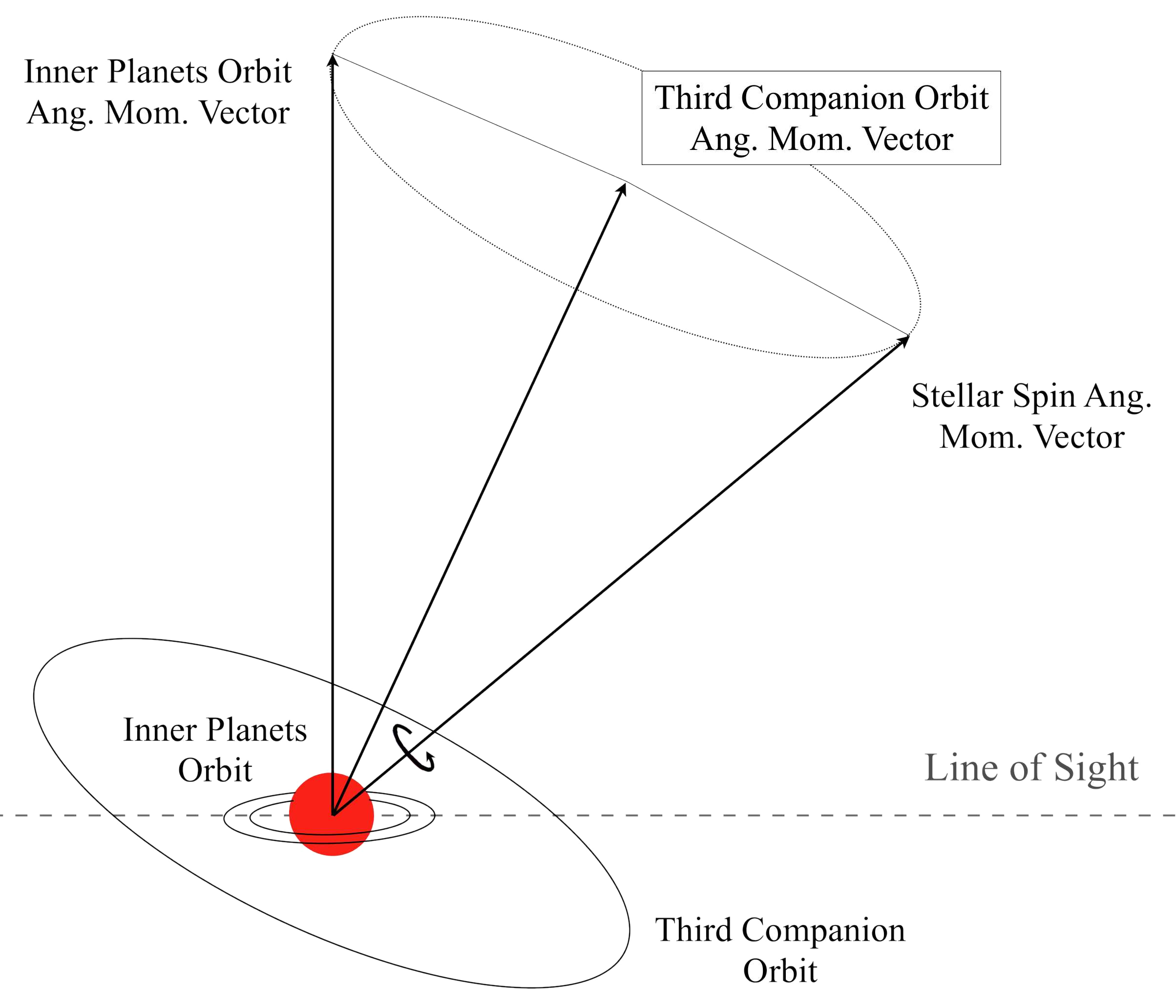
Kepler-56’s core and envelope
rotate around different axes.
(Ong 2025)
Zvrk rotates too fast to
not have eaten something recently.
(Ong et al. 2024)
8 UMi b should have
been consumed, but wasn’t?
(Hon+ 2023 incl. Ong)
In the data-rich régime,
technique development and
theoretical interpretation are
rate-limiting steps to discovery.

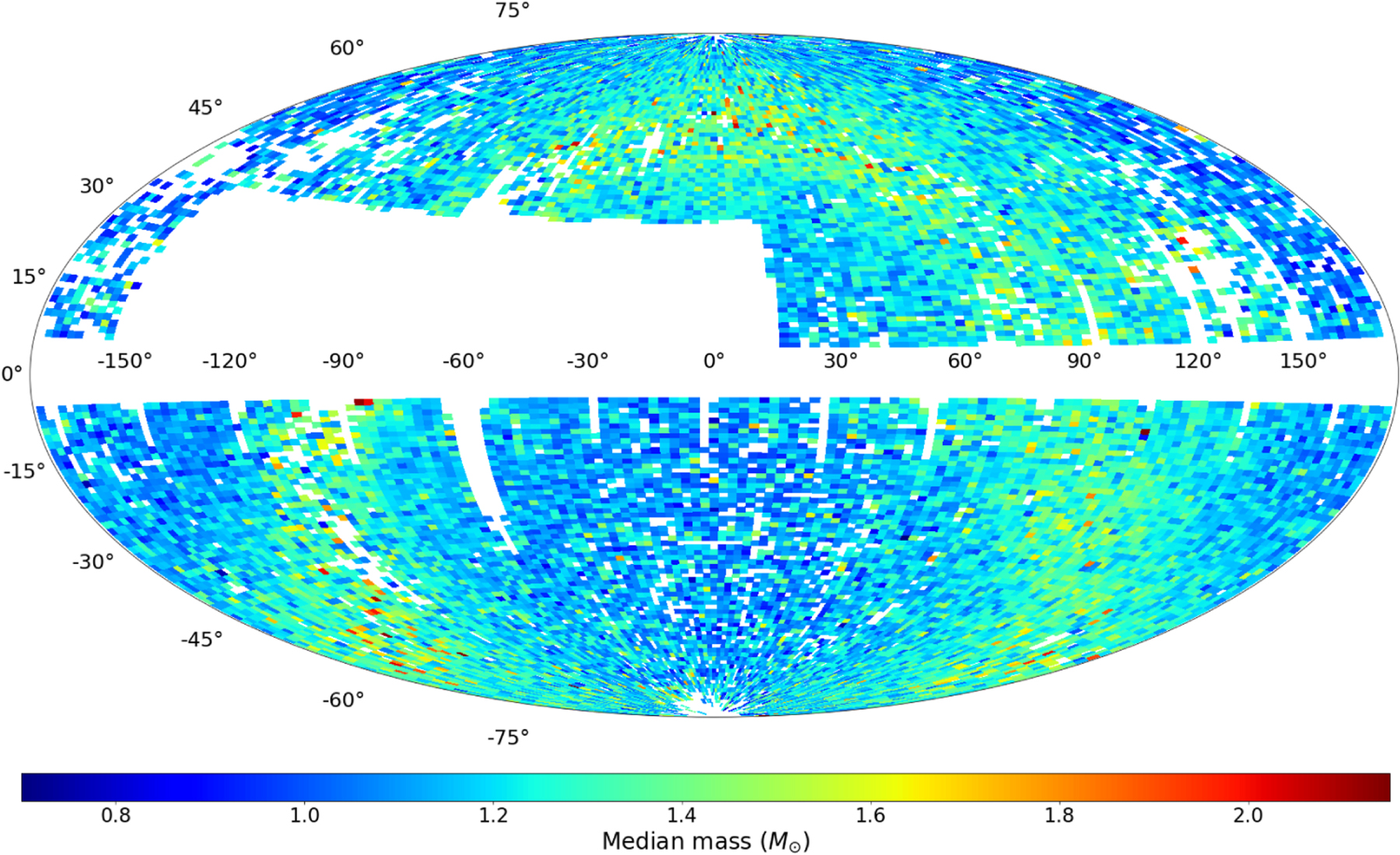
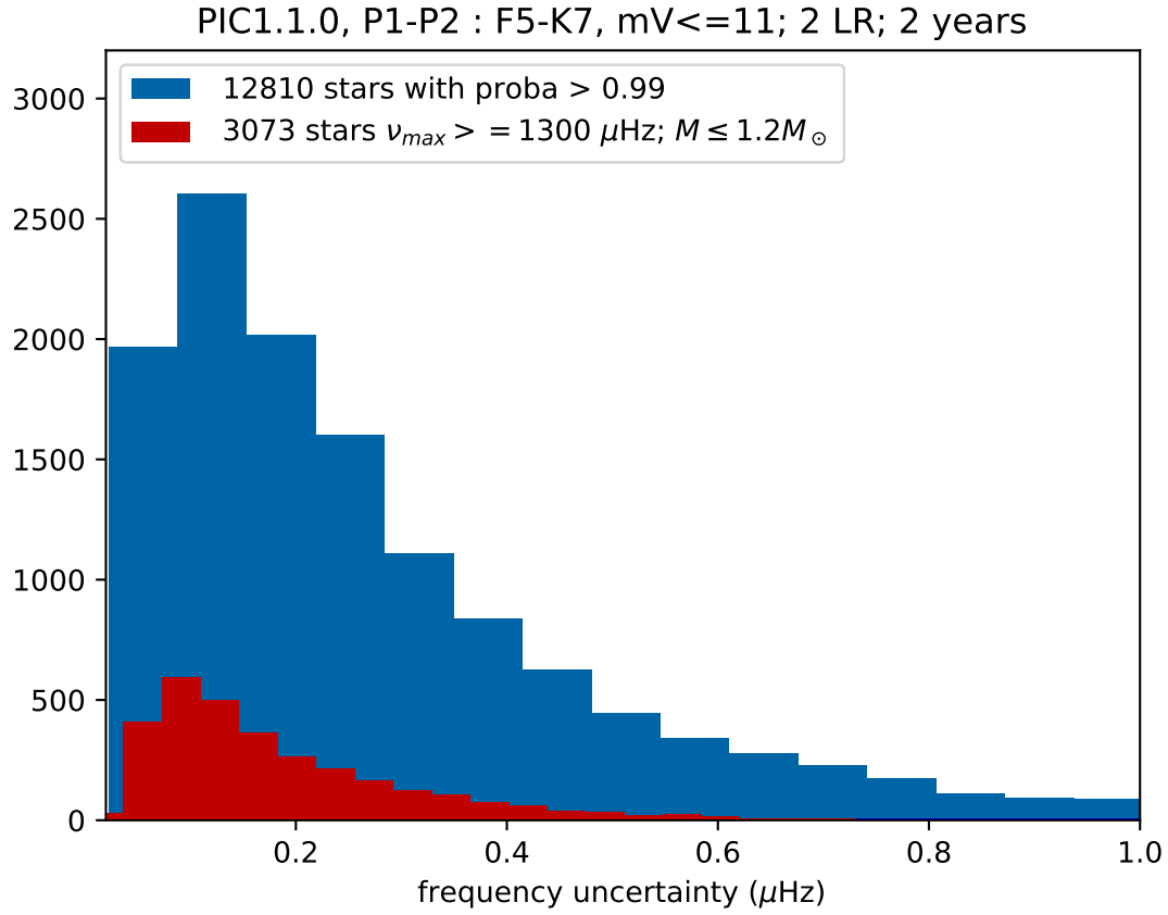
Statistical sample (Ong: WP 120, 128)
\(\sim 10^6\) red giants in galactic bulge & globular clusters
Long temporal baselines
(Ong: TASOC WG1, WG2, WG7)
\(\sim100 \to 10,000++\)
stars:
How do we cope with
a deluge of new data?
e.g. Hey, Huber, Ong, et al. in review;
Nielsen, Ong, et al., in review.
(incl. Ong: Cunha+ 2021; Nielsen+
2021; Campante+ 2023)
Ong: TASOC WG1, WG2; PLATO WP120, 128
?
Combining with Photometric surveys —
e.g. Ong et al. (2024); Hart+
incl. Ong (2023) 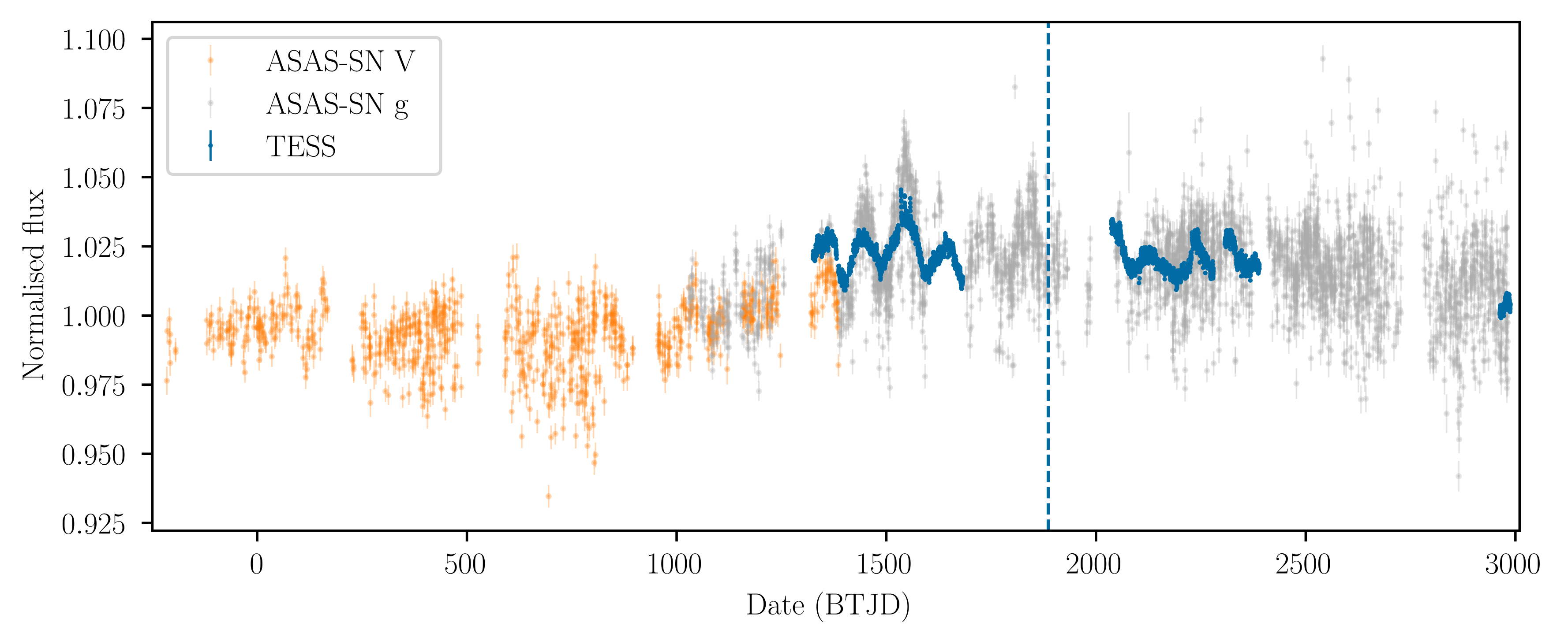
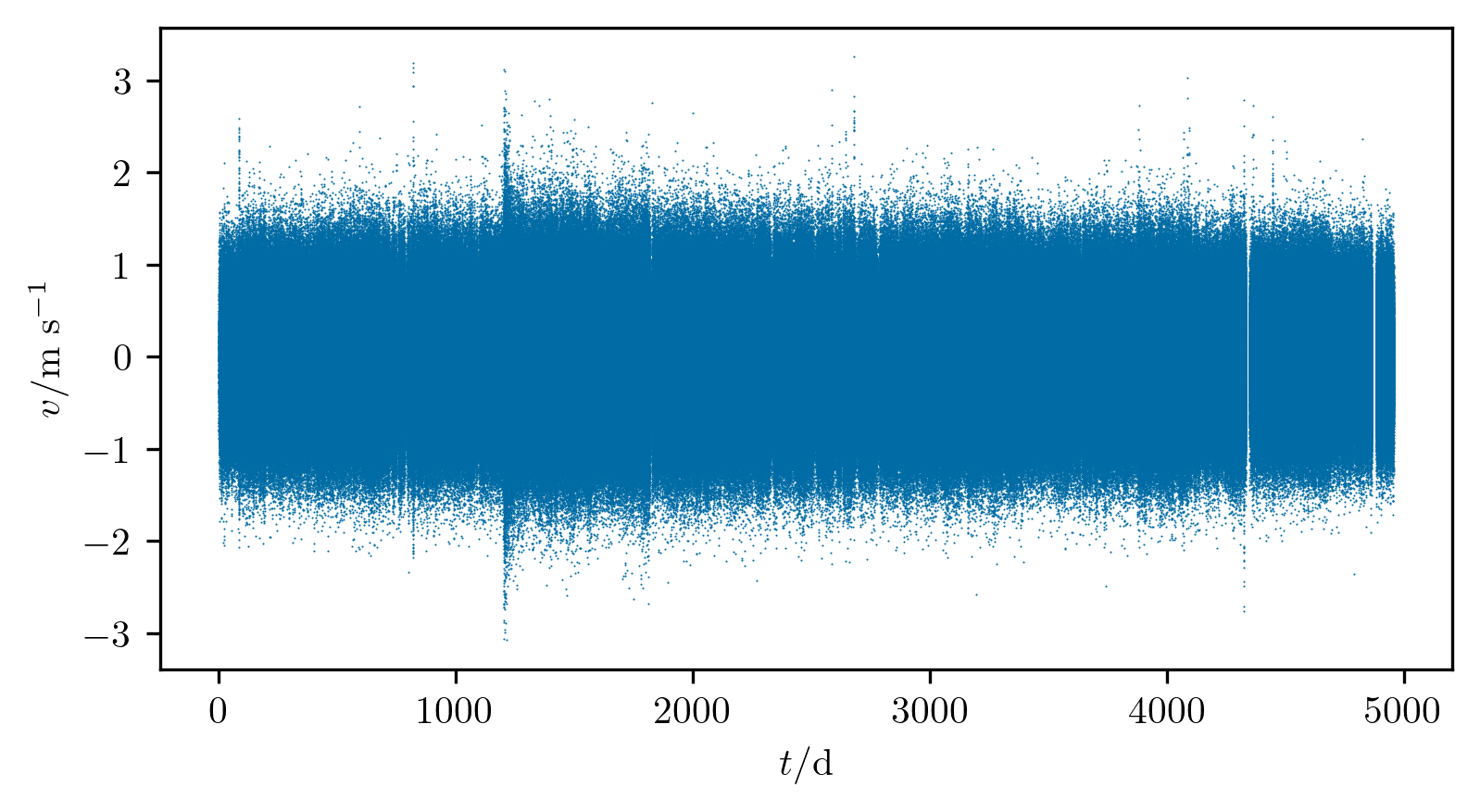
Seismology from Extreme Precision Radial Velocities
(Li, Huber, Ong, et al. 2025; Hon+ incl. Ong 2024) 
Ong: ASAS-SN; SONG WG1 & WG2; Keck Planet Finder via CPS
Coming Soon: HARPS-N; MINERVA; Rubin/LSST; G-CLEF?
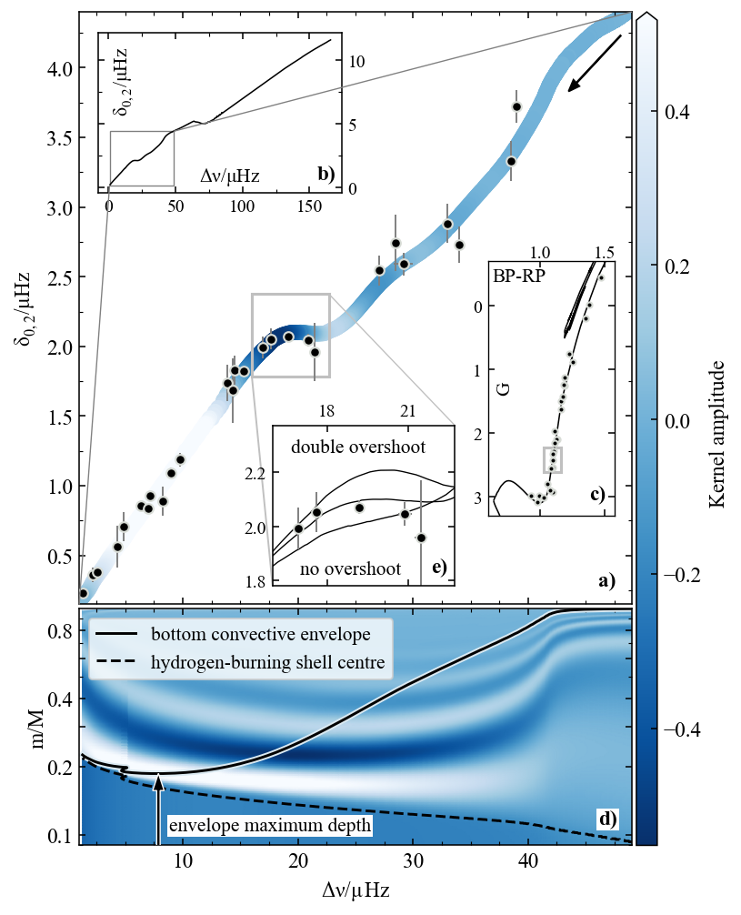
Probes of mixing processes
near convective boundaries
(Lindsay, Ong, Basu 2022†, and
2024†;
Ong, Lindsay, Reyes et al. 2025;
Reyes, Stello, Ong, et al. 2025†, Nature)


†: mentoree paper

Ong: TESS Guest Investigator Cycle 7, PI
?
Nonlinear evolution is
the primary obstacle to
g-mode inversions.
Will understanding this (Hoogendam, Ong, in prep.†) permit further technique development?


proxy for age \(\to\)
†: mentoree paper

The Sun as seen by SOHO:
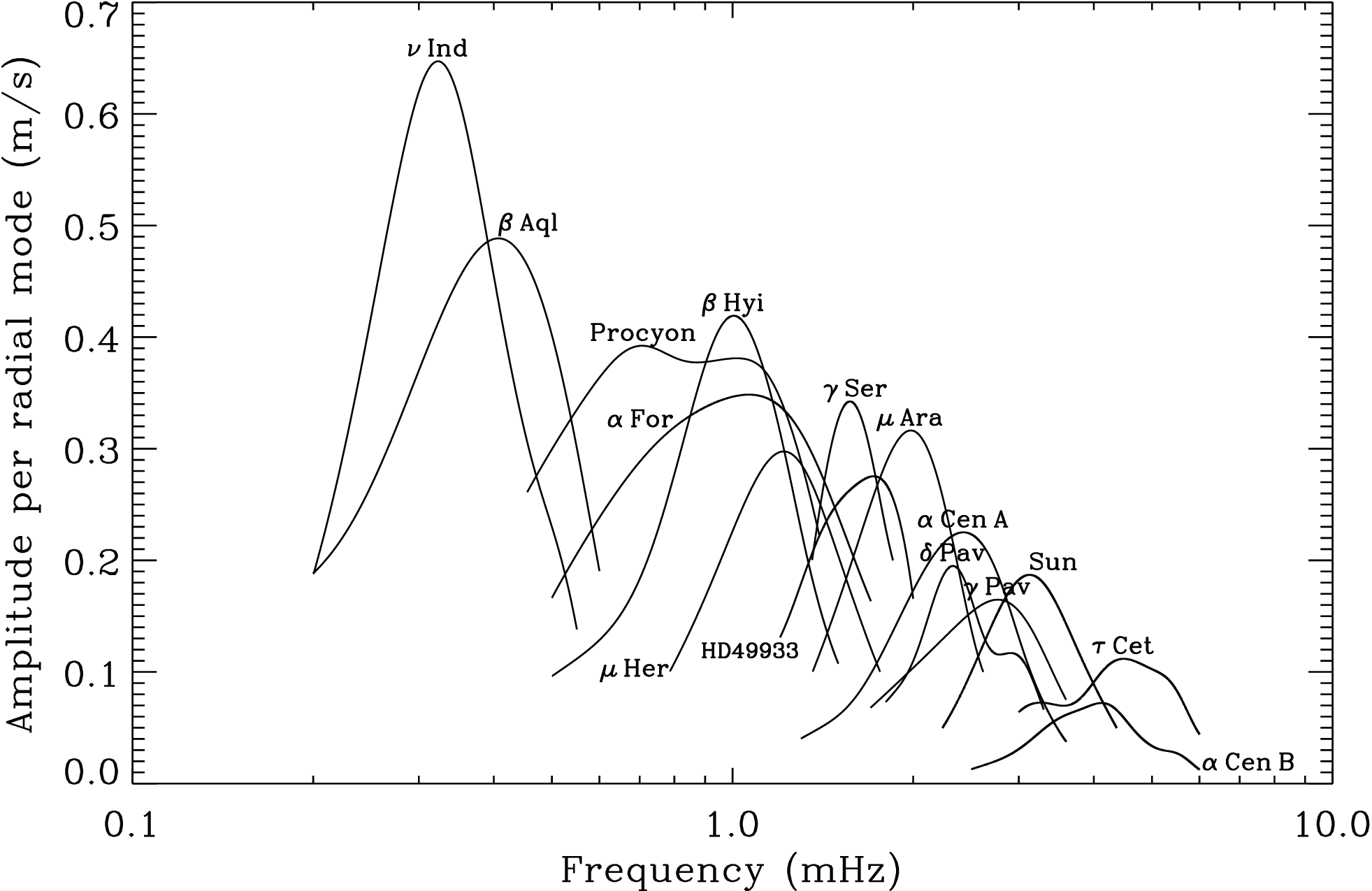
Bedding & Kjeldsen 2005

Procyon from MOST vs. RVs:
Huber et al. 2011


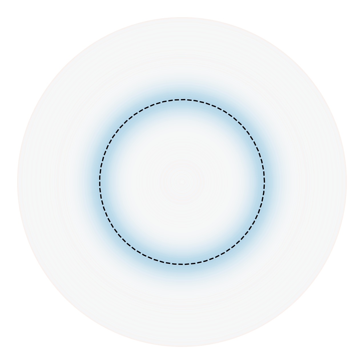
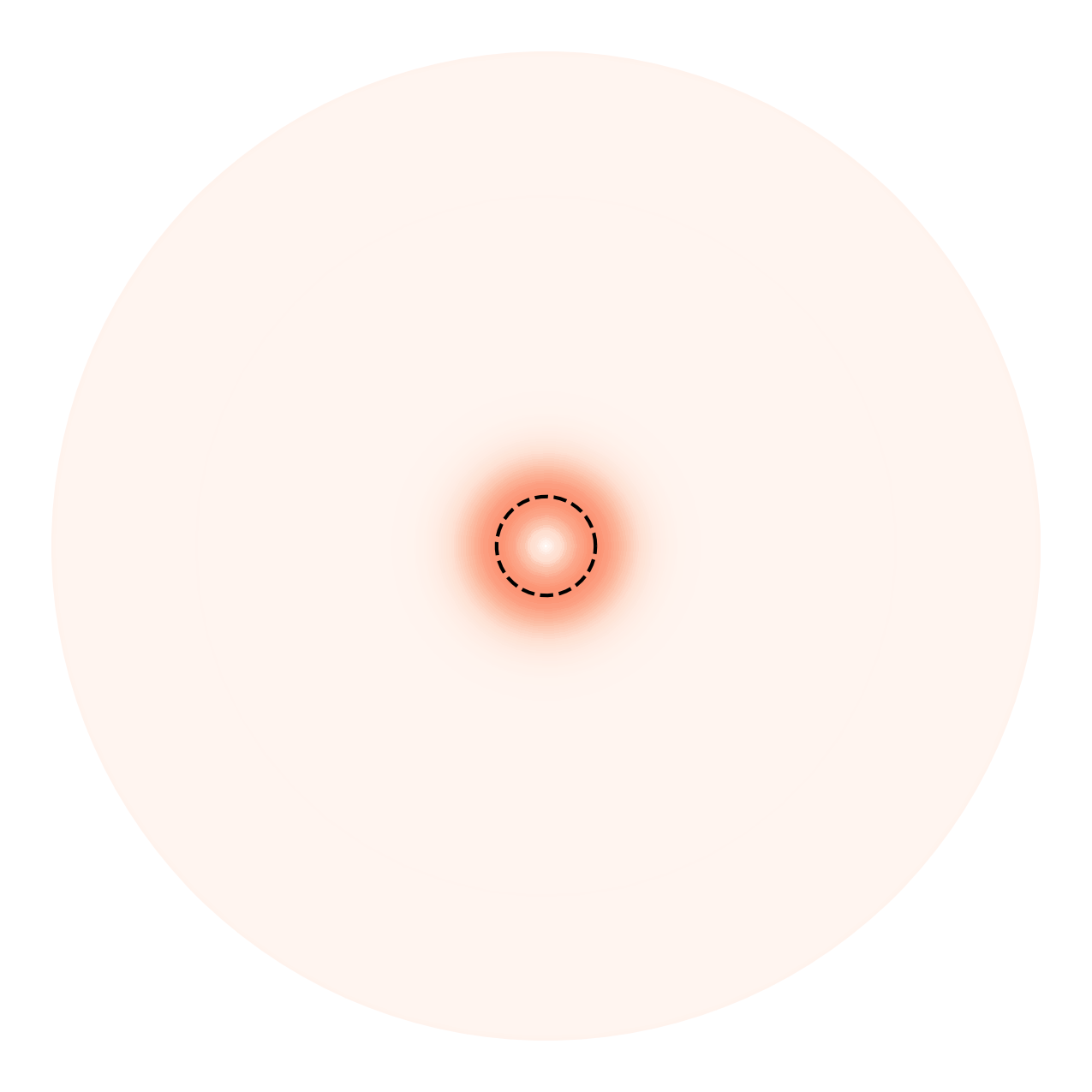
For slow rotation, \[\boxed{\delta\omega_{nlm} \sim m b_{nl} \int \Omega(r) K_{nl}(r) \mathrm d r}\]
Variations in \(\delta\omega_\text{rot}\) are
radial differential rotation.
\[\boxed{{\color{orange}{\delta\omega_{nlm}}} \sim {\color[RGB]{0,100,255}{m b_{nl} \sum_i {\color{black}{\Omega(r_i)}} K_{nl}(r_i) \Delta r_i}}}\] is of the form \({\color[RGB]{0,100,255}\mathbf{A}}\mathbf{x} = {\color{orange}\mathbf{b}}\).
i.e. Inferring the rotational profile
\(\Omega(r)\) is a linear
inverse problem.
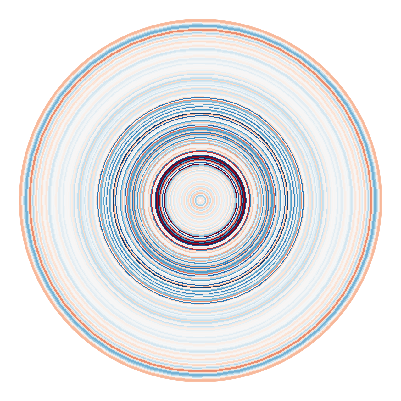
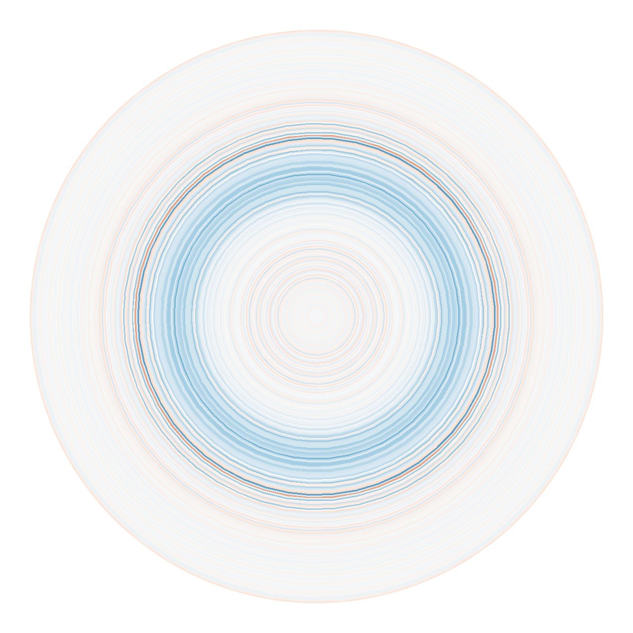
Rotational Inversions
\[\scriptsize\begin{aligned} \int \Omega(r) {\color[RGB]{0,100,255}\left(\sum_i c_i K_{i}(r)\right)} \mathrm d r &\sim \sum_{i} \left(c_i \over m_i b_{i} \right) \delta\omega_{\mathrm{rot}, i} \\ & \to \boxed{\Omega({\color[RGB]{0,100,255}r_0})}\end{aligned}\]
e.g. OLA
(Backus & Gilbert 1968; Gough 1985;
Pijpers & Thompson 1992; Schunker 2016; Ong 2024;
etc.)
\(\implies\) we can make measurements of internal rotational structure!
two standard
solar models
\[\huge {{\color{orange}{\delta\omega_i \over \omega_i}} \approx {\color[RGB]{0,100,255}{\int K_{\rho|c_s^2, i}(r)}} {\delta\rho \over \rho}{\color[RGB]{0,100,255}{\mathrm d r}} + {\color[RGB]{0,100,255}{\int K_{c_s^2|\rho, i}(r)}} {\delta c_s^2 \over c_s^2}{\color[RGB]{0,100,255}{\mathrm d r}}} \]
\[{\Large{\color[RGB]{0,100,255}\mathbf{A}}\mathbf{x} = {\color{orange}\mathbf{b}}}\]
Structure perturbations
do not reorder mixed modes!
(cf. Ball+ 2018)


Mode mixing yields avoided crossings
between multiplet components of identical \(m\)
(cf. Mosser+ 2012, Ouazzani+ 2013, Deheuvels+ 2017)
pure p
pure g
mixed
Very high \(\mathrm{A(Li)}\),
but otherwise innocuous


\[\ell = 0,2?\]
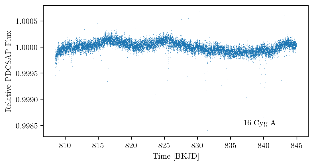
But Kepler says \(\ell =
0\) have to live here!
(and theory says so too…)
Rotational splittings from seismology:


\(\implies P_\text{rot} \sim 115\ \mathrm{d}?\)
Rotational signal probably got
detrended away
by systematic corrections…

Very suggestive…
but is this real?

Probably yes!


Gaia RV scatter rules out
large RV semiamplitudes…
\(P_\text{orb} \gg 99\ \mathrm{d}\)
cannot spin star
up to 99-day rotational period…
Remaining permissible orbits are
unstable to tidal dissipation!
\(\implies\) ENGULFMENT?
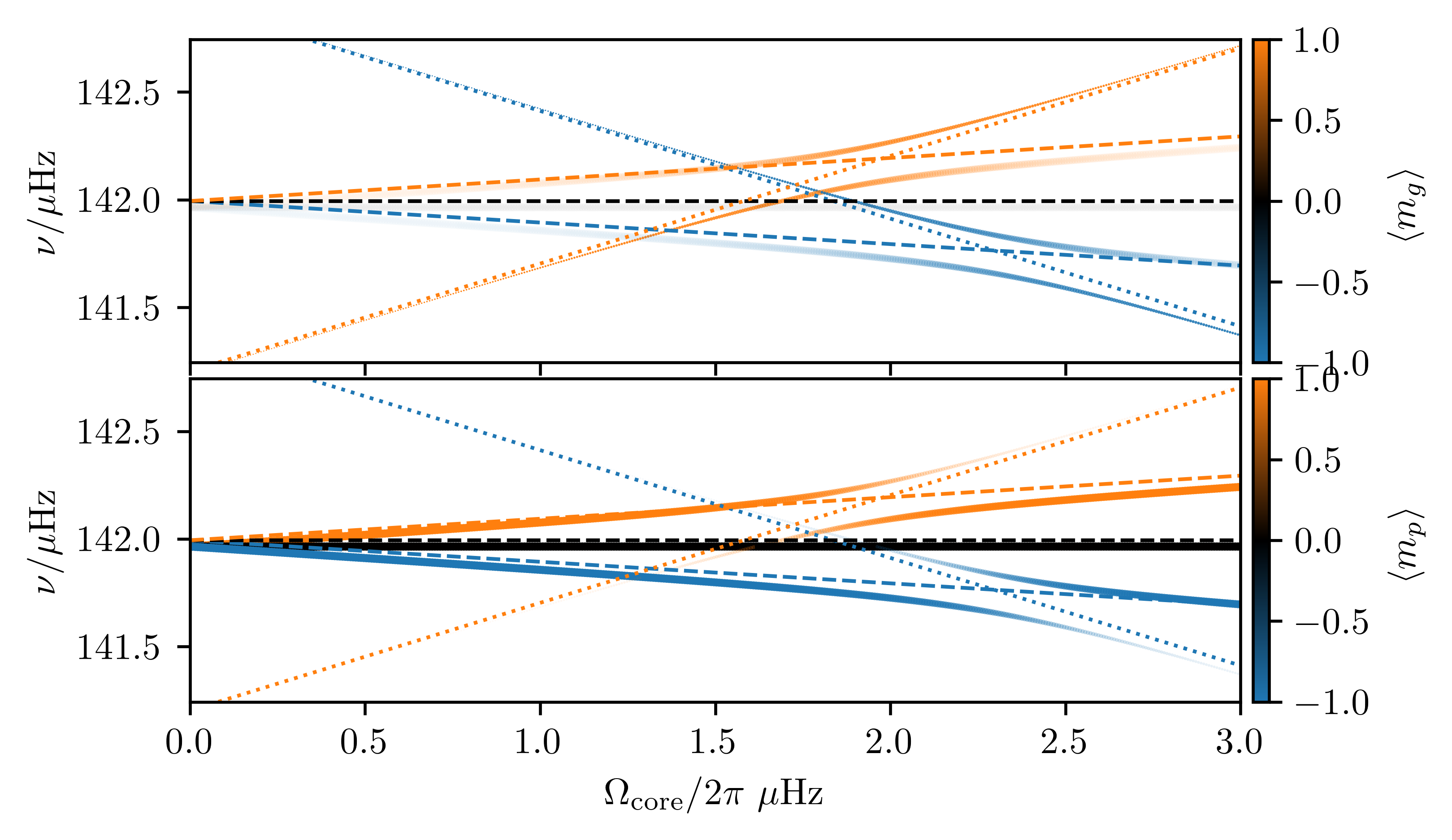
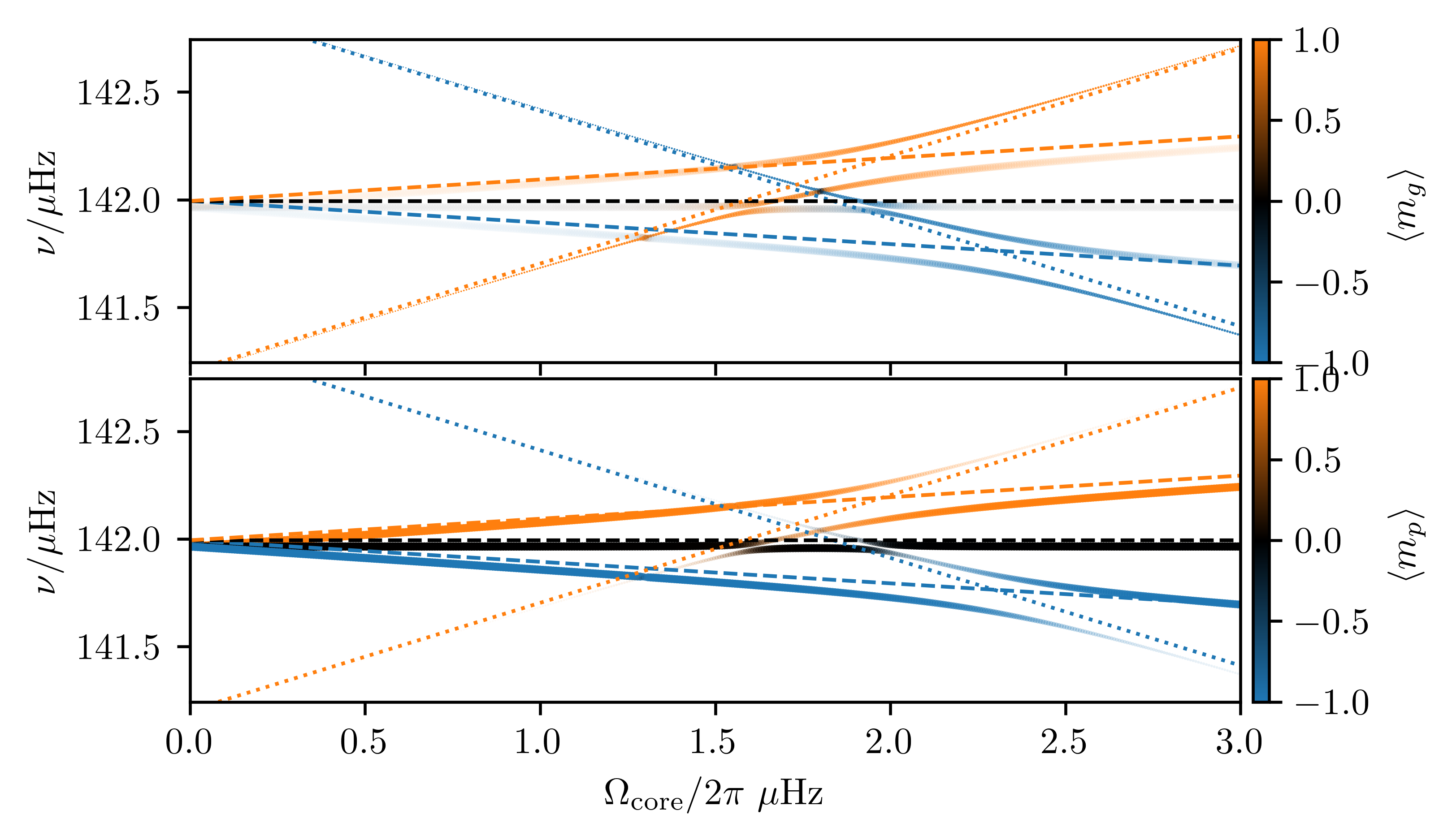
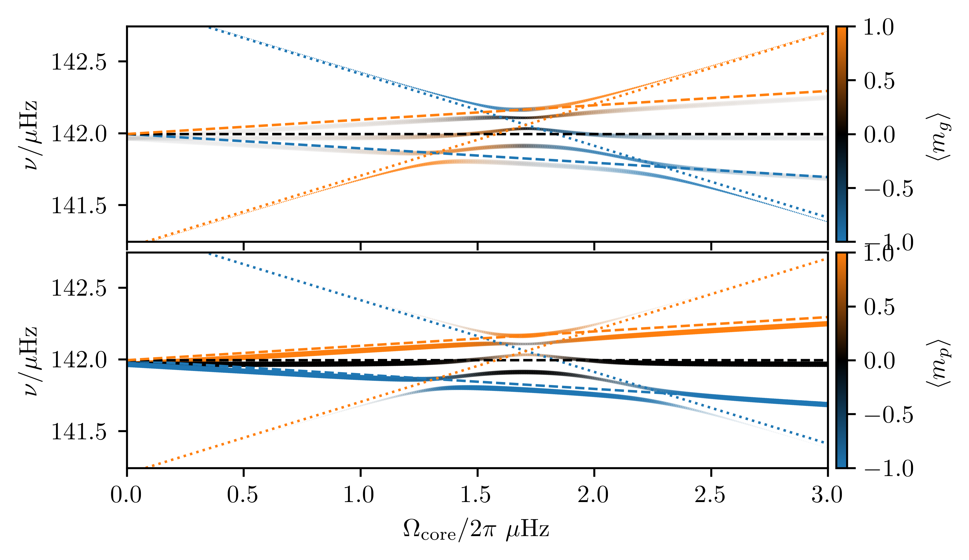
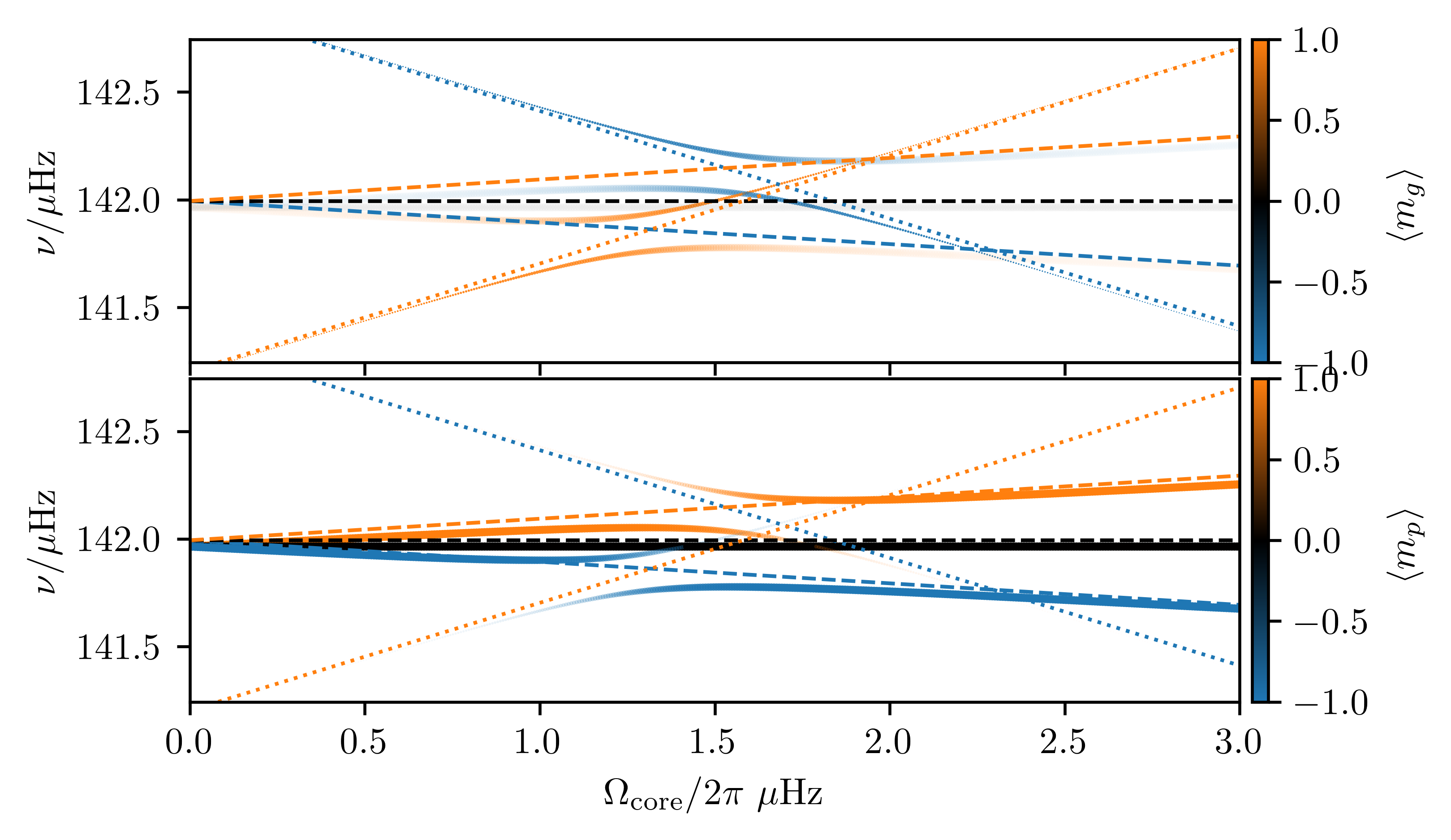
\(\beta = 0\)
\(\beta = {\pi\over10}\)
\(\beta = {\pi\over2}\)
\(\beta = \pi\)